Linear Regression: A Mathematical and Practical Guide with NumPy

What is Linear Regression?

Linear regression is a fundamental statistical method used for modeling the relationship between a dependent variable and one or more independent variables. It's a type of linear approach to modeling the relationship between a dependent variable and one or more independent variables. The case of one independent variable is called simple linear regression; for more than one, the process is called multiple linear regression.

In simple linear regression, the relationship between the independent variable $$x$$ and the dependent variable $$y$$ is modeled as a straight line. The goal is to find the best-fitting line that describes the relationship between the variables. This line is represented by the equation $$y = mx + b$$

where:

• $$y$$ = dependent variable or the one we want to predict.
• $$x$$ = independent variable or the one we use to make predictions.
• $$m$$ = slope of the line, which represents the change in slope for one unit change in $$x$$
• $$b$$ = the y-intercept which is the value of $$y$$ when $$x = 0$$

The values of $$m$$ and $$b$$ are determined during the training phase of the linear regression model. The model is trained using a dataset pairs of $$x$$ and $$y$$ values. The training process involves finding the values of $$m$$ and $$b$$ that minimizes the differences between actual $$y$$ values in the dataset and the $$y$$ values predicted by the model.

Once the model is trained, it can be used to make predictions on new data by plugging the new $$x$$ values into the equation $$y = mx+b$$. The model will then output the predicted $$y$$ values based on the input $$x$$ values.

Types of Linear Regression

In the context of machine learning and statistical modeling, linear regression can be classified into several types based on the number of independent variables and the nature of the relationships they represent. Here are some common types of linear regression:

1. Simple Linear Regression:

• Simple linear regression involves only one independent variable. The relationship between the independent variable $$x$$ and the dependent variable $$y$$ is modeled as a straight line.
• The equation for simple linear regression is $$y = mx + b$$, where $$m$$ is the slope of the line and $$b$$ is the y-intercept.

1. Multiple Linear Regression:

• Multiple linear regression involves more than one independent variable. The relationship between the dependent variable $$y$$ and multiple independent variables $$x1, x2, ..., xn$$ is modeled as a linear combination of these variables.
• The equation for multiple linear regression is $$y = b_0 + b^1x_1 + b^2x_2 + ... + b^nx_n$$ where $$b_0$$ is the intercept, and $$b^1, b^2, ..., b^n$$ are the coefficients for the independent variables.

1. Polynomial Regression:

• Polynomial regression is a type of regression analysis in which the relationship between the independent variable $$x$$ and the dependent variable $$y$$ is modeled as an $$n$$-degree polynomial.
• The equation for polynomial regression is $$y = b_0 + b^1x + b_2x^2 + ... + b_nx^n$$, where $$b_0, b^1, ..., b^n$$ are the coefficients of the polynomial terms.

1. Ridge Regression:

• Ridge regression is a variation of linear regression that includes a regularization term in the loss function. This regularization term helps to prevent overfitting by penalizing large coefficient values.
• Ridge regression is particularly useful when dealing with multicollinearity (high correlation between independent variables) in multiple linear regression.

1. Lasso Regression:

• Lasso regression, like ridge regression, is a regularization technique that adds a penalty term to the loss function. However, lasso regression uses the L1 norm of the coefficient vector as the penalty term, which can lead to sparse solutions (i.e., some coefficients may become exactly zero).
• Lasso regression is often used for feature selection in high-dimensional datasets.

1. ElasticNet Regression:

• ElasticNet regression is a combination of ridge and lasso regression. It uses a penalty term that is a mix of both L1 and L2 norms, allowing it to benefit from the strengths of both regularization techniques.

These are some of the common types of linear regression used in machine learning and statistics. Each type has its own advantages and is suitable for different types of data and modeling tasks.

Let's get to real deal

The Math behind Linear Regression

To understand the mathematics involved, I recommend going through the previous two blog posts where we discussed gradient descent and cost functions. They will be helpful.

Hypothesis Function

The hypothesis function in linear regression is a linear equation that represents the relationship between the independent variable ($$x$$) and the dependent variable ($$y$$). The equation is given by:

it's same as the one we discussed earlier in this post.

Here, \theta_{0}{:eq} is intercept and \theta_{1}{:eq} is the slope of the line

Cost Function

The cost function measures how well the hypothesis function predicts the actual values (In our case, it gives us the best fit line). In linear regression, the cost function is often the mean squared error (MSE), given by:

error = (predicted - actual)$$^2$$

this gives the error for just one data point.

We may have multiple data points, in which case we sum up the errors at every data point to obtain the total error.

and average of all

for mathematical convenience, we multiply the above equation with $$\frac{1}{2}$$. When we take the derivative of the cost function $$J(\theta)$$ with respect to the parameters $$\theta$$ for the purpose of gradient descent, the $$\frac{1}{2}$$ cancels out with the power of 2 in the squared error term, simplifying the derivative calculation.

Gradient Descent

We use gradient descent to update the parameters \theta_{0}{:eq} and \theta_{1}{:eq} to minimize the cost function:

We repeat this process until the cost converges to a minimum. Once we have the optimized parameters \theta_{0}{:eq} and \theta_{1}{:eq}, we can use the hypothesis function to make predictions for new values.

Let's implement this using Python from scratch.

Python Implementation

let's import the required libraries

import numpy as np
import matplotlib.pyplot as plt
import os
import imageio

now let's implement the linear regression

class LinearRegression:
    def __init__(self, lr:float=0.01, iters:int=300) -> None:
        self.lr = lr
        self.iters = iters
        self.weights = None
        self.bias = None
        
        
    def fit(self, X:np.ndarray, y:np.ndarray, **kwargs) -> None:
        n_samples, n_features = X.shape
        self.weights = np.zeros(n_features)
        self.bias = 0
        
        if 'plot_dir' in kwargs:
            self.plot_dir = kwargs['plot_dir']
            
            os.makedirs(self.plot_dir, exist_ok=True)
        
        for i in range(self.iters):
            y_pred = self.predict(X)
            
            dw = (1/n_samples) * np.dot(X.T, (y_pred - y))
            db = (1/n_samples) * np.sum(y_pred - y)
            
            # updating the weights
            self.weights = self.weights - self.lr * dw
            self.bias = self.bias - self.lr * db
            
            # optional (for plotting at each epoch)
            if 'plot_dir' in kwargs:
                plt.figure(figsize=(8, 8))
                plt.scatter(X, y, color="b", label="Actual")
                plt.plot(X, y_pred, color="r", label="Predicted")
                plt.title(f"Epoch: {i}, Weight: {self.weights[0]:.3f}, bias: {self.bias:.3f}")
                plt.legend()
                plt.savefig(f"{self.plot_dir}/{i}_plot.png")
                plt.close()

    def predict(self, X:np.ndarray) -> np.ndarray:
        return np.dot(X, self.weights) + self.bias
    
    def make_gif(self):
        images = [imageio.imread(f"{self.plot_dir}/{x}_plot.png") for x in range(self.iters)]
        imageio.mimsave("lr_gif.gif", images)

let's prepare some data for linear regression

from sklearn.datasets import make_regression
from sklearn.model_selection import train_test_split

X, y = make_regression(n_samples=1000, n_features=1, noise=20, random_state=42)
X_train, X_test, y_train, y_test = train_test_split(X, y, test_size=0.2, random_state=42, shuffle=True)

let's have a look at the first 10 samples from X and y below

| X | y | |--------|---------------| | -1.758739 | -36.084949 | | 1.031845 | -10.272417 | | -0.487606 | -27.694060 | | 0.186454 | -11.103187 | | 0.725767 | 14.055202 | | 0.972554 | 51.280219 | | 0.645376 | -23.945672 | | 0.681891 | 49.248252 | | -1.430141 | -8.350814 | | 1.066675 | -4.097966 |

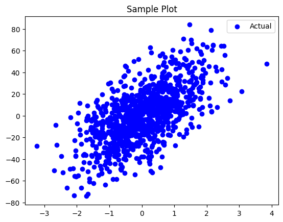
if we plot all the data points, this is how it looks

plt.scatter(X, y, color="b", label="Actual")
plt.legend()
plt.title("Sample Plot")

let's train our model

reg = LinearRegression(iters=500)
reg.fit(X_train, y_train, plot_dir='linear_reg_plots')
y_pred = reg.predict(X_test)

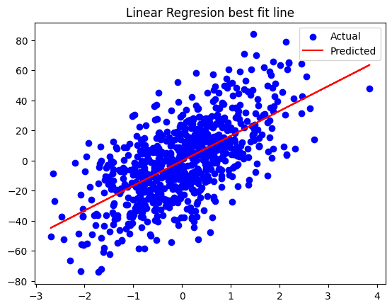
if we plot the best fit line after training

plt.scatter(X_train, y_train, color="b", label="Actual")
plt.plot(X_train, y_pred, color="r", label="Predicted")
plt.title("Linear Regresion best fit line")
plt.legend()

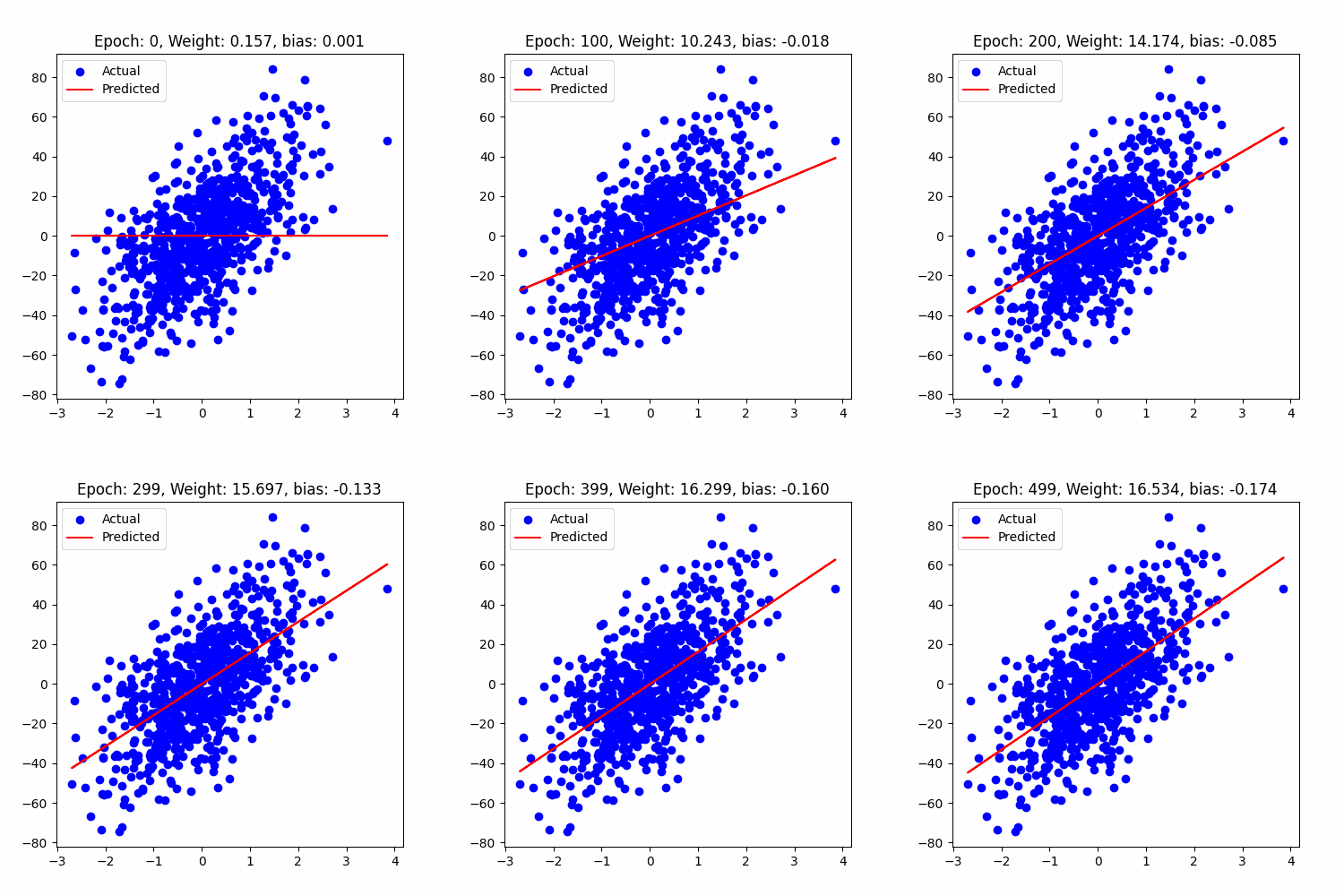
let's have a look at how our model performed

Comparision with Standard Library

let's compare our model with standard library, scikit-learn

from sklearn import linear_model
from sklearn.metrics import mean_absolute_error, mean_squared_error, r2_score

lr = linear_model.LinearRegression()
lr.fit(X_train, y_train)
y_pred_sk = lr.predict(X_train)

if we compare the error metrics on test data for both models, we get

Our Model (Scratch):

mae = mean_absolute_error(y_test, y_pred)
mse = mean_squared_error(y_test, y_pred)
rmse = np.sqrt(mse)
r_squared = r2_score(y_test, y_pred)

# Print the error metrics
print("Mean Absolute Error (MAE):", mae)
print("Mean Squared Error (MSE):", mse)
print("Root Mean Squared Error (RMSE):", rmse)
print("R-squared (R2):", r_squared)

the output is:

Mean Absolute Error (MAE): 16.340180822972712
Mean Squared Error (MSE): 431.3609648508903
Root Mean Squared Error (RMSE): 20.769231205099775
R-squared (R2): 0.37607990198934305

Scikit-Learn Model:

mae = mean_absolute_error(y_test, y_pred_sk)
mse = mean_squared_error(y_test, y_pred_sk)
rmse = np.sqrt(mse)
r_squared = r2_score(y_test, y_pred_sk)

# Print the error metrics
print("Mean Absolute Error (MAE):", mae)
print("Mean Squared Error (MSE):", mse)
print("Root Mean Squared Error (RMSE):", rmse)
print("R-squared (R2):", r_squared)

and the output is:

Mean Absolute Error (MAE): 16.34302989576724
Mean Squared Error (MSE): 431.59967479663885
Root Mean Squared Error (RMSE): 20.774977131073786
R-squared (R2): 0.3757346321460251

as we see, the error metrics are almost close to each other.

In the next post we will discuss about the polynomial regression and how it's different from Linear Regression.